ORBE orbital integrator


ascl:1702.001
Version 3, September 2016.
Numerical integration of an arbitrary planetary system composed by a central star and up to 100 planets and minor bodies.
For educational purposes only.
This program is presented in "Exploring the orbital evolution of planetary systems", T. Gallardo 2017, European Journal of Physics, Vol 38 (3). Preprint here.
CHARACTERISTICS
  • Designed to be used in the classroom to explore the long term orbital dynamics of planetary systems and minor bodies.
  • Very simple usage. One plain text file with the initial conditions and one plain text output file with the results of the simulation.
  • Integrates forward or backward in time.
  • Code available in Fortran. Compilations for Windows, Linux and Mac OS.
  • Installation: does not need installation. Just download ORBE for Windows, Linux or Mac OS, decompress and put the files in a folder.

    RESTRICTIONS
  • Maximum number of objects = 100. Can be changed manipulating the code.
  • Not precise for objects that are experiencing close encounters.
  • ORBITAL ELEMENTS

    ORBE calculates the orbital evolution of a system of bodies by means of the computation of the time evolution of their orbital elements. It does not generate the cartesian coordinates (x,y,z) because in the long term evolution, that means millions of years, the positions are not relevant, only the orbital elements are. It is a very simplified and limited version of EVORB (by A. Brunini and T. Gallardo). On the other hand it is a version of very easy usage, suitable for being used by undergraduate students in the classroom as a first approach to orbital integrators.

    The 6 orbital elements are:
    • a: semimajor axis of the ellipse in astronomical units
    • e: eccentricity of the ellipse (between 0 and 1, 0 is a circle)
    • i: inclination of the orbit in degrees (from 0 to 180, 0 if is coincident with plane xy or ecliptic, 90 perpendicular, 180 retrograde motion)
    • Omega: longitude of the ascending node in degrees (from 0 to 360, 0 corresponds to Aries or x-axis)
    • omega: argument of the perihelion in degrees (from 0 to 360, 0 corresponds to the direction of the node)
    • M: mean anomaly in degrees (from 0 to 360, 0 corresponds to perihelion, 180 to aphelion)
    and the mass must be given in solar masses or 0 in case of "particles", that means real or fictitious minor bodies.
    ?
    USAGE:
    
                                                                                        gnuplot
    orbeini.dat ------> orbe.exe -------> orbeout.dat  (time, object, orbital elements) -------> figures
    (edit with          (run with         (edit with Notepad or Textpad)
      Notepad          double click)
     or Textpad)


    1) FIRST STEP: prepare orbeini.dat

    Put in the same folder the executable file orbe.exe and the input data orbeini.dat. Edit orbeini.dat with a plain text editor (Notepad, TextPad) and indicate the details of the simulation:
    1. mass of the central star in solar masses (1 for the Sun)
    2. final time of the numerical integration in years. For integrations to the past put a negative number.
    3. interval for output data. For a 1 Myr integration, an output of 500 or 1000 yrs is ok.
    4. orbital elements and mass for each particle in the order a, e, i, longitude of the node, argument of the perihelion, mean anomaly, mass separated by space

    Example of orbeini.dat:
    
    *MASS OF THE STAR IN SOLAR MASSES
    1
    *YEARS FROM PRESENT TO END THE SIMULATION
    -1000000
    *INTERVAL FOR OUTPUT DATA IN YEARS
    1000
    *ORBITAL ELEMENTS: a e i node w M mass (in solar masses)
       0.387098  0.205640   7.00   48.32  29.14 143.52 0.1660136E-06
       0.723329  0.006759   3.39   76.66  54.53  24.82 0.2447838E-05
       0.999988  0.016717   0.00  175.41 287.62 257.61 0.3040432E-05
       1.523674  0.093437   1.85   49.54 286.56 226.11 0.3227155E-06
       5.202040  0.048933   1.30  100.51 274.18 223.70 0.9547919E-03
       9.551249  0.054508   2.49  113.63 340.06  38.63 0.2858859E-03
      19.176263  0.048094   0.77   73.96  98.52 169.39 0.4366244E-04
      30.098703  0.006894   1.77  131.78 264.31 283.25 0.5151389E-04
    
    	
    In this example we integrate the Solar System (form Mercury to Neptune) with the Sun (mass = 1) at the center from the present to 1 Myr to the past with output of the state of the system each 1000 years.
    Semimajor axes, a, must be expressed in astronomical units.
    Inclination, longitude of the node, argument of the perihelion and initial mean anomaly must be expressed in degrees.
    Mass of each object must be expressed in solar masses. For fictitious particle put m = 0.
    Do not eliminate the four lines with comments beginning with an asterisk (*).

    2) SECOND STEP: run orbe.exe

    Execute orbe.exe (with double click or by typing in a terminal) and wait. In the screen you will see the progress of the integration. Once the program ends you can explore the output file orbeout.dat using the same text editor you used for orbeini.dat. You can kill the program with CTRL-C. The larger the number of objects, the larger the computation time. If the output interval is small the file orbeout.dat will be larger, take care. If there is an object with small semimajor axis (Mercury for example) the integration slows down.

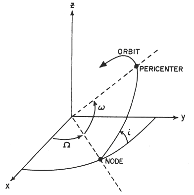
    3) THIRD STEP: analyze orbeout.dat

    Here is an extract of the file orbeout.dat
    
    -5.000000E+05   1     0.387099 0.213741   8.10  70.56  24.99 288.30
    -5.000000E+05   2     0.723323 0.017668   4.00 107.96 124.98 103.19
    -5.000000E+05   3     1.000012 0.034443   1.24  91.78  88.26  79.11
    -5.000000E+05   4     1.523737 0.055313   5.03 180.79 162.97  48.72
    -5.000000E+05   5     5.203247 0.027860   1.60  97.19  53.54 268.17
    -5.000000E+05   6     9.513984 0.079794   2.05 135.20  26.11  70.25
    -5.000000E+05   7    19.249354 0.059683   1.84  73.28 297.28 343.09
    -5.000000E+05   8    30.125651 0.005854   0.92 105.64 218.39 171.68
    
       time       planet    a        e         i    node     w      M
    
    
    This extract corresponds to the state of the system at t=-500000 yrs. Using your favorite program plot the orbital elements as funtion of the time. We recommend gnuplot. Excel is not a good tool for plotting scientific data. Here is the script of gnuplot used to generate the figure:
    
    set terminal png
    set output "orbe2.png"
    set size 0.8, 1
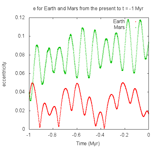
    set title "e for Earth and Mars from the present to t = -1 Myr"
    set xlabel "Time (Myr)"
    set ylabel "eccentricity"
    p [-1:0][] "orbeout.dat" u ($1/1e6):($2==3 ? $4 : 1/0) w p ps 0.2 title "Earth" , \
    "orbeout.dat" u ($1/1e6):($2==4 ? $4 : 1/0) w p ps 0.2 title "Mars"
    
    
    and this simple script shows in the screen a,e,i,nodes,w:
    
    p [][] "orbeout.dat" u 1:3 w p ps 0.1
    pause -1
    p [][] "orbeout.dat" u 1:4 w p ps 0.1
    pause -1
    p [][] "orbeout.dat" u 1:5 w p ps 0.1
    pause -1
    p [][] "orbeout.dat" u 1:6 w p ps 0.1
    pause -1
    p [][] "orbeout.dat" u 1:7 w p ps 0.1
    pause -1
    
    
    At present (t=0) Mars' eccentricity (e=0.093) is larger than Earth's eccentricity (e=0.016). But in the past (t=-950000 yrs) the Earth was more eccentric than Mars. Both e(t) seems to be the addition of some periodic terms, try to obtain the spectrum of them. Plotting e(t) is just the beginning, try to plot other elements and for all planets.
    ?

    SOME PROJECTS FOR THE CLASSROOM

    • Integrate the Solar System to the past and to the future by 1 Myr with output 1000 yrs and plot the orbital elements a(t), e(t), i(t) for all planets.
    • Repeat but assuming the central star has mass = 0.5
    • Integrate only the giant planets Jupiter, Saturn, Uranus and Neptune by 1 Myr. Change a little the initial semimajor axis or eccentricity of one planet and compare with the original system. How much can we change the planets before the system becomes unstable?
    • Integrate the giant planets plus a fictitious planet with mass 0.0001 in an orbit between Jupiter and Saturn. Look for stable and unstable configurations.
    • Consider only Jupiter and a planet (try mass 0.0001) coorbital (same a) with Jupiter but with initial M = M_J + 180. It is an unstable configuration.
    • Repeat but with initial M = M_J + 60. They will be trapped in a stable configuration.
    • Explore the dynamics of a high inclination particle. Kozai mechanism will show up.
    • Can the Earth have a twin? Put an extra Earth with different initial mean anomaly M and run.
    • What happens if we put a new planet between Venus and Earth?
    • Dynamical memory of comet Halley. Integrate backwards the giant planets plus Halley and some clones. Plot a(t) for the Halleys and determine up to when we can know the past of the comet.
    • Nemesis. What happens to the Solar System if we add an extra Jupiter like planet in a very large and eccentric orbit?
    • The TRAPPIST-1 system. Try to follow the orbital evolution of this famous system of 7 planets
    • Test the hypothesis of planet 9 according to Batygin and Brown 2016.
    • Use your imagination...
    See the input files for these projects here.

    Orbital elements

    Other orbital integrators

    Auxiliary software

    CONTACT
    Tabare Gallardo
    gallardo@fisica.edu.uy